Table Outer Join
Description
Use, as you might have expected, to perform a full outer join operation on 2 data tables, combining them into a single data table based upon the join key(s) specified.
For more details on outer join methodology, see here: Wikipedia SQL Full Outer Join
Table Data Selection
Table Source
Specify the source data table by selecting it from the dropdown menu.
Source Columns
Specify any columns to be included here. Selecting the Inspect Source and Populate Source Mapping Table buttons will make these columns available for the join operation.
Select Subset of Source Data
Any valid Python expression is acceptable to subset the data. Please see Expressions for more details and examples.
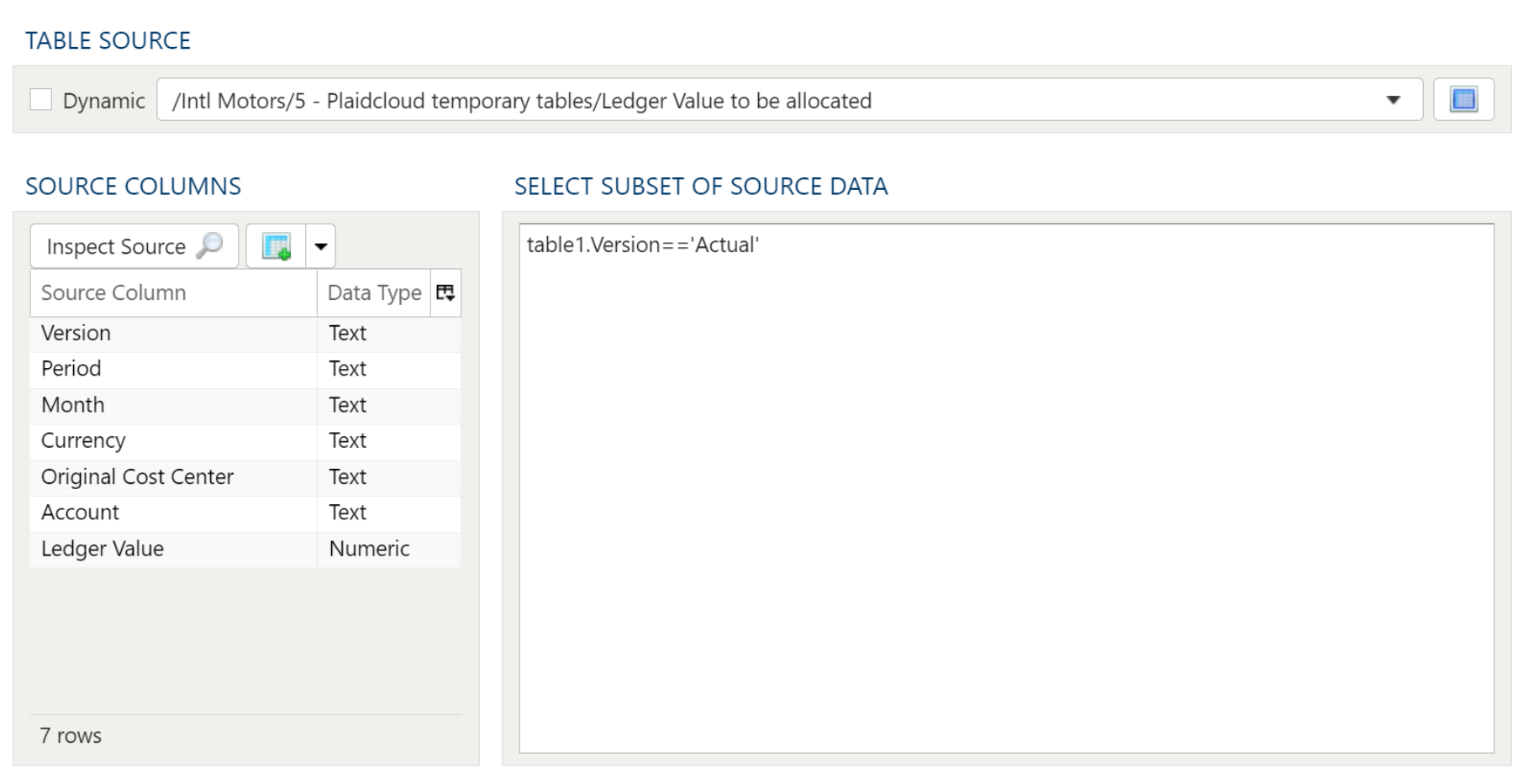
Table Output
Target Table

To establish the target table select either an existing table as the target table using the Target Table dropdown or click on the green "+" sign to create a new table as the target.
Table Creation
When creating a new table you will have the option to either create it as a View or as a Table.
Views:
Views are useful in that the time required for a step to execute is significantly less than when a table is used. The downside of views is they are not a useful for data exploration in the table Details mode.
Tables:
When using a table as the target a step will take longer to execute but data exploration in the Details mode is much quicker than with a view.
Join Map
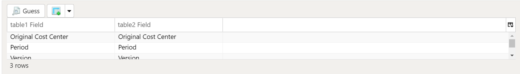
Specify join conditions. Using the Guess button will find all matching columns from both Table 1 as well as Table 2. To add additional columns manually, right click anywhere in the section and select either Insert Row or Append Row, to add a row prior to the currently selected row or to add a row at the end, respectively. Then, type the column names to match from Table 1 to Table 2. To remove a field from the Join Map, simply right-click and select Delete.
Target Output Columns
Data Mapper Configuration
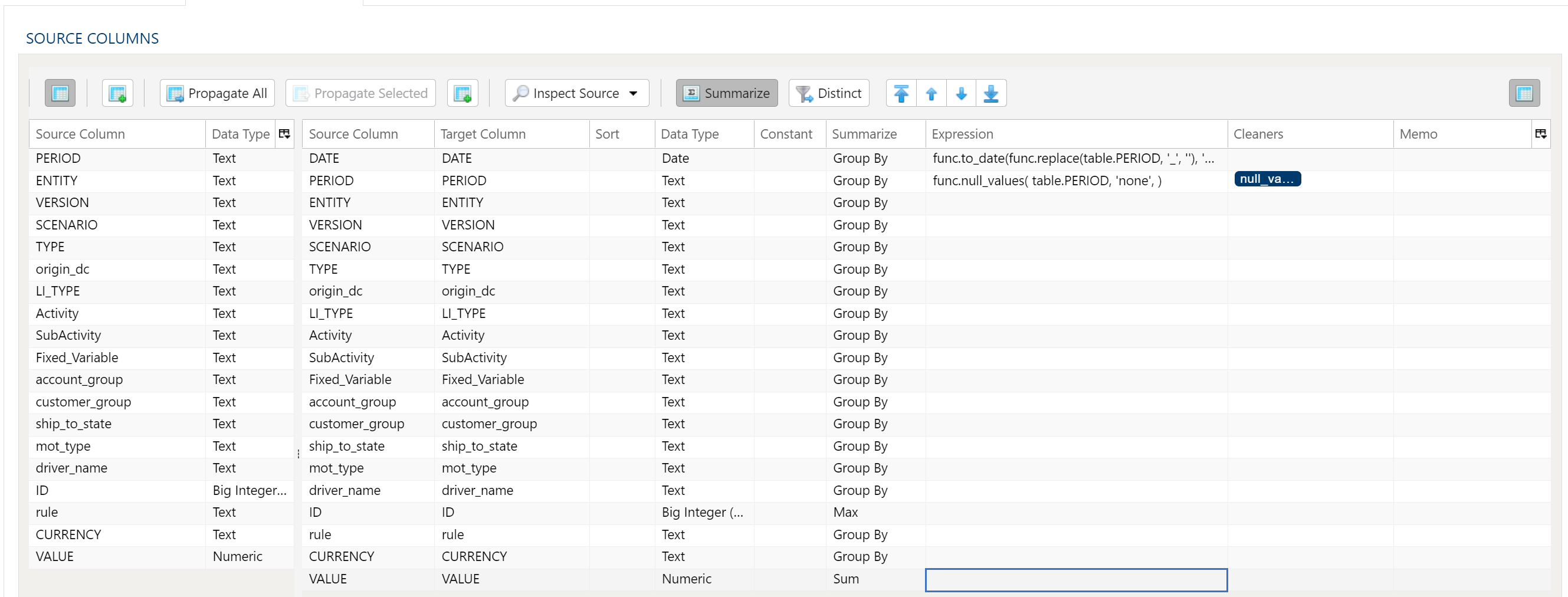
The Data Mapper is used to map columns from the source data to the target data table.
Inspection and Populating the Mapper
Using the Inspect Source menu button provides additional ways to map columns from source to target:
- Populate Both Mapping Tables: Propagates all values from the source data table into the target data table. This is done by default.
- Populate Source Mapping Table Only: Maps all values in the source data table only. This is helpful when modifying an existing workflow when source column structure has changed.
- Populate Target Mapping Table Only: Propagates all values into the target data table only.
If the source and target column options aren’t enough, other columns can be added into the target data table in several different ways:
- Propagate All will insert all source columns into the target data table, whether they already existed or not.
- Propagate Selected will insert selected source column(s) only.
- Right click on target side and select Insert Row to insert a row immediately above the currently selected row.
- Right click on target side and select Append Row to insert a row at the bottom (far right) of the target data table.
Deleting Columns
To delete columns from the target data table, select the desired column(s), then right click and select Delete.
Chaging Column Order
To rearrange columns in the target data table, select the desired column(s). You can use either:
- Bulk Move Arrows: Select the desired move option from the arrows in the upper right
- Context Menu: Right clikc and select Move to Top, Move Up, Move Down, or Move to Bottom.
Reduce Result to Distinct Records Only
To return only distinct options, select the Distinct menu option. This will toggle a set of checkboxes for each column in the source. Simply check any box next to the corresponding column to return only distinct results.
Depending on the situation, you may want to consider use of Summarization instead.
The distinct process retains the first unique record found and discards the rest. You may want to apply a sort on the data if it is important for consistency between runs.
Aggregation and Grouping
To aggregate results, select the Summarize menu option. This will toggle a set of select boxes for each column in the target data table. Choose an appropriate summarization method for each column.
- Group By
- Sum
- Min
- Max
- First
- Last
- Count
- Count (including nulls)
- Mean
- Standard Deviation
- Sample Standard Deviation
- Population Standard Deviation
- Variance
- Sample Variance
- Population Variance
- Advanced Non-Group_By
For advanced data mapper usage such as expressions, cleaning, and constants, please see the Advanced Data Mapper Usage
Output Filters
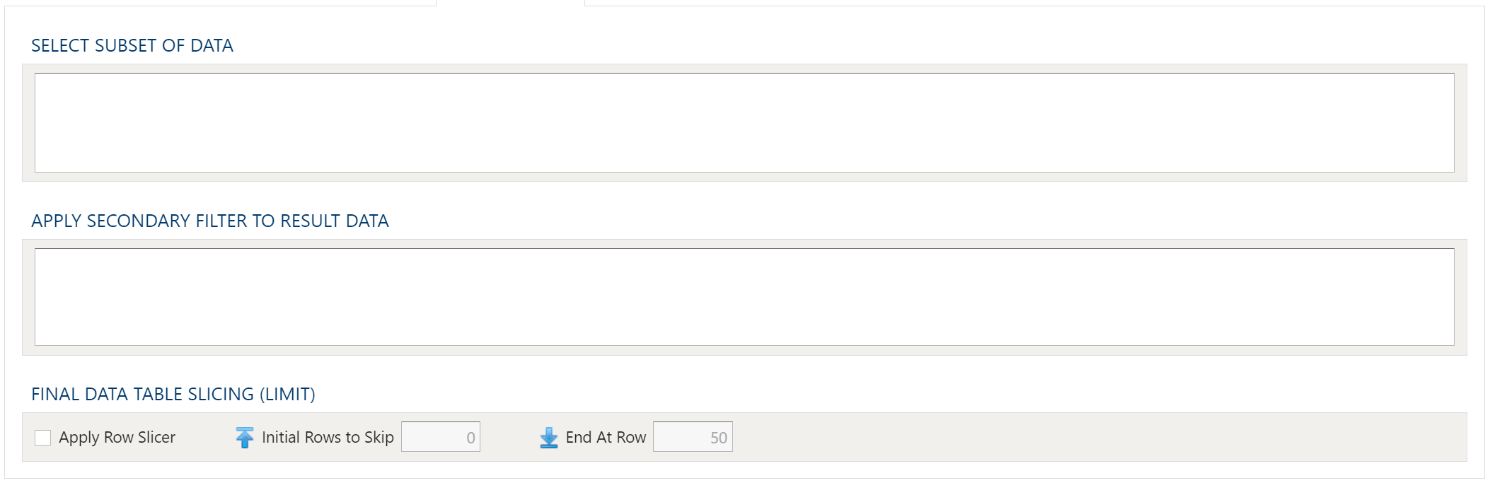
To allow for maximum flexibility, data filters are available on the source data and the target data. For larger data sets, it can be especially beneficial to filter out rows on the source so the remaining operations are performed on a smaller data set.
Select Subset Of Data
This filter type provides a way to filter the inbound source data based on the specified conditions.
Apply Secondary Filter To Result Data
This filter type provides a way to apply a filter to the post-transformed result data based on the specified conditions. The ability to apply a filter on the post-transformed result allows for exclusions based on results of complex calcuations, summarizaitons, or window functions.
Final Data Table Slicing (Limit)
The row slicing capability provides the ability to limit the rows in the result set based on a range and starting point.
Filter Syntax
The filter syntax utilizes Python SQLAlchemy which is the same syntax as other expressions.
View examples and expression functions in the Expressions area.
Examples
Join Automobile Manufacturers with Models
In this example, consider the following source data tables. First is a list of automobile manufacturers.
| Mfg_ID | Manufacturer |
|---|---|
| 1 | Aston Martin |
| 2 | Porsche |
| 3 | Lamborghini |
| 4 | Ferrari |
| 5 | Koenigsegg |
Next is a list of automobile models with a manufacturer ID. Note that there are several models with no manufacturer.
| ModelName | Mfg_ID |
|---|---|
| Aventador | 3 |
| Countach | 3 |
| DBS | 1 |
| Enzo | 4 |
| One-77 | 1 |
| Optimus Prime | |
| Batmobile | |
| Agera | 5 |
| Lightning McQueen |
To get a list of models by manufacturer, it makes sense to join on Mfg_ID. By leveraging outer join concepts, the output will also be able to show those items which do not have any matches.
First, specify parameters for Table 1 Data Selection. The source data table is selected and all columns are listed.
Next, specify parameters for Table 2 Data Selection. Once again, the source data table is selected and all columns are listed.
Finally, the join conditions are set in the Table Output tab. Using the Guess button, Analyze properly identifies the Mfg_ID column to use as the Join Key. Lastly, the
Target Output Columns are specified automatically using the Propagate button. This effectively includes all columns from all tables, with any join columns obviously only being included a single time. Note that the columns are sorted alphabetically, first by Manufacturer and next by ModelName.
As expected, the final output includes all rows from both tables, whether they had a match in both tables or not. As such, this time Porsche does indeed show up despite having no models. Additionally, Batmobile, Lightning McQueen, and Optimus Prime are included in the results even though none of them have a manufacturer. Besides, who can say ‘No’ to them?